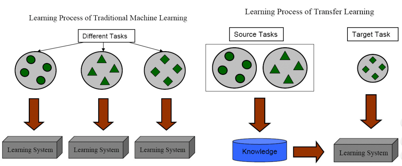
Domain adaptation (DA) is transfer learning which aims to leverage labeled data in a related source domain to achieve informed knowledge transfer and help the classification of unlabeled data in a target domain.
Machine learning vs Transfer learning
Notation Table
Symbol
Notation
Defintion
$\mathcal{D}$
Domain
$$\mathcal{D}=\{\mathcal{X}, \mathcal{P}(x)\}$$
$\mathcal{X}$
Feature space
$$\mathcal{X}=\{x_1, x2, ..., x_N\}$$
$\mathcal{P}$
Marginal Probability
Probability of any single event occurring unconditioned on any other events. Whenever someone asks you whether the weather is going to be rainy or sunny today, you are computing a marginal probability.
$T$
Task
$$T=\{\mathcal{Y}, f(x)\}$$
$\mathcal{Y}$
Label
Label Set
$f(x)$
Conditional probability function for input x
$$f(x)=\mathcal{Q}(y|x)$$
$\mathcal{S}$
Source
$$S=\{x_i,y_i\}$$
Problem Statement
Given with $\mathcal{D}_\mathcal{S}$, where S has label information, how to infer another domain $\mathcal{D}_\mathcal{T}$'s label set, i.e. $\mathcal{Y_T}$? Suppose that :
Our Proposals
In short, our proposals are based on two principals:
P1: Find a new latent feature space, where the distance of $\mathcal{P}(\mathcal{X_S})$ and $ \mathcal{P}(\mathcal{X_T})$ is minimized;
P2: Infer $\mathcal{Q}(\mathcal{Y_T|X_T})$ by prior information in $\mathcal{Q}(\mathcal{Y_S|X_S})$ in sprit of semi-supervised paradigm.
(I) First, to follow P1 and P2, we explicitely minimize the discrepancy between the source and target domain, measured in terms of both marginal and conditional probability distribution via Maximum Mean Discrepancy is minimized so as to attract two domains close to each other.
(II) Second, to follow P1 and P2, we also design a repulsive force term, to explicitely minimize the discrepancy between the subdomain of source and target domain;
(III) Finally, to follow P2, we infer the label set of target domain by label space gometric smoothless
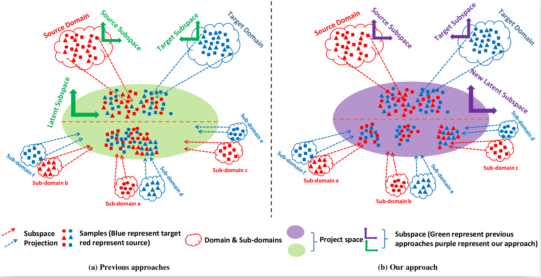
Overview
Illustration of the major difference between our proposed method and previous state-of-the-art: The geometrical shape in round, triangle and square represents samples of different class labels. Cloud colored in red or blue represents the source or target domain, respectively. The latent shared feature space is represented by ellipse. The green ellipse illustrates the the latent feature space obtained by the previous approaches, whereas the purple one illustrates the novel latent shared feature space by the proposed method. The upper part of both ellipses represents the marginal distribution, while the lower part denotes the conditional distribution. As can be seen from the marginal distribution in the lower part of Fig.1(b), samples with same label are clustered together while samples with different labels, thus from different sub-domains, are separated. This is in contrast with the conditional distribution in the lower part of Fig.1(a) where samples with different labels are completely mixed, thus making harder the discrimination of samples of different labels
Algorithm
Closer: Marginal and Conditional Distribution Domain Adaptation
Marginal Distribution Domain Adaptation:
$$Dis{t^{marginal}}({{\cal D}_{\cal S}},{{\cal D}_{\cal T}}) =\\ {\left\| {\frac{1}{{{n_s}}}\sum\limits_{i = 1}^{{n_s}} {{{\bf{A}}^T}{x_i} - } \frac{1}{{{n_t}}}\sum\limits_{j = {n_s} + 1}^{{n_s} + {n_t}} {{{\bf{A}}^T}{x_j}} } \right\|^2}
= tr({{\bf{A}}^T}\bf{X}{\bf{M_0}}\bf{{X^T}A}) $$
where ${{\bf{M}}_0}$ represents the marginal distribution between ${{\cal D}_{\cal S}}$ and ${{\cal D}_{\cal T}}$ and its calculation is obtained by:
$$\begin{array}{l}
{({{\bf{M}}_0})_{ij}} = \left\{ \begin{array}{l}
\frac{1}{{{n_s}{n_s}}},\;\;\;{x_i},{x_j} \in {D_{\cal S}}\\
\frac{1}{{{n_t}{n_t}}},\;\;\;{x_i},{x_j} \in {D_{\cal T}}\\
0,\;\;\;\;\;\;\;\;\;\;\;\;otherwise
\end{array} \right.
\end{array}$$
Conditional Distribution Domain Adaptation:
the sum of the empirical distances over the class labels between the sub-domains of a same label in the source and target domain
$$\begin{array}{c}
\begin{array}{l}
Dis{t^{conditional}}\sum\limits_{c = 1}^C {({{\cal D}_{\cal S}}^c,{{\cal D}_{\cal T}}^c)} = \\
{\left\| {\frac{1}{{n_s^{(c)}}}\sum\limits_{{x_i} \in {{\cal D}_{\cal S}}^{(c)}} {{{\bf{A}}^T}{x_i}} - \frac{1}{{n_t^{(c)}}}\sum\limits_{{x_j} \in {{\cal D}_{\cal T}}^{(c)}} {{{\bf{A}}^T}{x_j}} } \right\|^2}\\
= tr({{\bf{A}}^T}{\bf{X}}{{\bf{M}}_c}{{\bf{X}}^{\bf{T}}}{\bf{A}})
\end{array}
\end{array}
$$
where $\bf M_c$ represents the conditional distribution between sub-domains in ${{\cal D}_{\cal S}}$ and ${{\cal D}_{\cal T}}$ and it is defined as:
$$
\begin{array}{*{20}{c}}
{{{({{\bf{M}}_c})}_{ij}} = \left\{ {\begin{array}{*{20}{l}}
{\frac{1}{{n_s^{(c)}n_s^{(c)}}},\;\;\;{x_i},{x_j} \in {D_{\cal S}}^{(c)}}\\
{\frac{1}{{n_t^{(c)}n_t^{(c)}}},\;\;\;{x_i},{x_j} \in {D_{\cal T}}^{(c)}}\\
{\frac{{ - 1}}{{n_s^{(c)}n_t^{(c)}}},\;\;\;\left\{ {\begin{array}{*{20}{l}}
{{x_i} \in {D_{\cal S}}^{(c)},{x_j} \in {D_{\cal T}}^{(c)}}\\
{{x_i} \in {D_{\cal T}}^{(c)},{x_j} \in {D_{\cal S}}^{(c)}}
\end{array}} \right.}\\
{0,\;\;\;\;\;\;\;\;\;\;\;\;otherwise}
\end{array}} \right.}
\end{array}
$$
Repulsive Force Domain Adaptation
The repulsive force domain adaptation is defined as:
$Dis{t^{repulsive}} = Dist_{{\cal S} \to {\cal T}}^{repulsive} + Dist_{{\cal T} \to {\cal S}}^{repulsive}$, where ${{\cal S} \to {\cal T}}$ and ${{\cal T} \to {\cal S}}$ index the distances computed from ${D_{\cal S}}$ to ${D_{\cal T}}$ and ${D_{\cal T}}$ to ${D_{\cal S}}$, respectively. $Dist_{{\cal S} \to {\cal T}}^{repulsive}$ represents the sum of the distances between each source sub-domain ${D_{\cal S}}^{(c)}$ and all the target sub-domains ${D_{\cal T}}^{(r);\;r \in \{ \{ 1...C\} - \{ c\} \} }$ except the one with the label $c$.
$${Dist}_{{\cal S} \to {\cal T}}^{repulsive} = \sum\limits_{c = 1}^C \begin{array}{l}
{\left\| {\frac{1}{{n_s^{(c)}}}\sum\limits_{{x_i} \in {D_{\cal S}}^{(c)}} {{{\bf{A}}^T}{x_i}} - \frac{1}{{\sum\limits_{r \in \{ \{ 1...C\} - \{ c\} \} } {n_t^{(r)}} }}\sum\limits_{{x_j} \in D_{\cal T}^{(r)}} {{{\bf{A}}^T}{x_j}} } \right\|^2}\\
= \sum\limits_{c = 1}^C {tr({{\bf{A}}^T}{\bf{X}}{{\bf{M}}_{{\cal S} \to {\cal T}}}{{\bf{X}}^{\bf{T}}}{\bf{A}})}
\end{array} $$
where ${{\bf{M}}_{{\cal S} \to {\cal T}}}$ is defined as:
$$
\begin{array}{c}
(\bf M_{{{\cal S} \to {\cal T}}})_{ij} = \left\{ {\begin{array}{*{20}{l}}
{\frac{1}{{n_s^{(c)}n_s^{(c)}}},\;\;\;{x_i},{x_j} \in {D_{\cal S}}^{(c)}}\\
{\frac{1}{{n_t^{(r)}n_t^{(r)}}},\;\;\;{x_i},{x_j} \in {D_{\cal T}}^{(r)}}\\
{\frac{{ - 1}}{{n_s^{(c)}n_t^{(r)}}},\;\;\;\left\{ {\begin{array}{*{20}{l}}
{{x_i} \in {\cal D_{\cal S}}^{(c)},{x_j} \in {D_{\cal T}}^{(r)}}\\
{{x_i} \in {\cal D_{\cal T}}^{(r)},{x_j} \in {\cal D_{\cal S}}^{(c)}}
\end{array}} \right.}\\
{0,\;\;\;\;\;\;\;\;\;\;\;\;otherwise}
\end{array}} \right.
\end{array}
$$
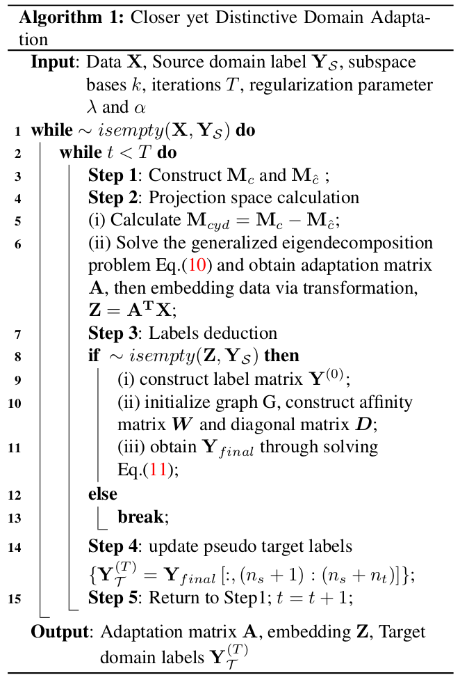
Optimization
The complete learning algorithm is summarized here
Experiment
For the problem of domain adaptation, it is not possible to tune a set of optimal hyper-parameters, given the fact that the target domain has no labeled data. Following the setting of JDA, we also evaluate the proposed CDDA by empirically searching the parameter space for the optimal settings. Specifically, the proposed CDDA method has three hyper-parameters, i.e., the subspace dimension $k$, regularization parameters $\lambda $ and $\alpha$.
In our experiments, we set $k = 100$ and 1) $\lambda = 0.1$, and $\alpha = 0.99$ for USPS, MNIST, COIL20 , 2) $\lambda = 0.1$, $\alpha = 0.2$ for PIE, 3) $\lambda = 1$, $\alpha = 0.99$ for Office and Caltech-256.
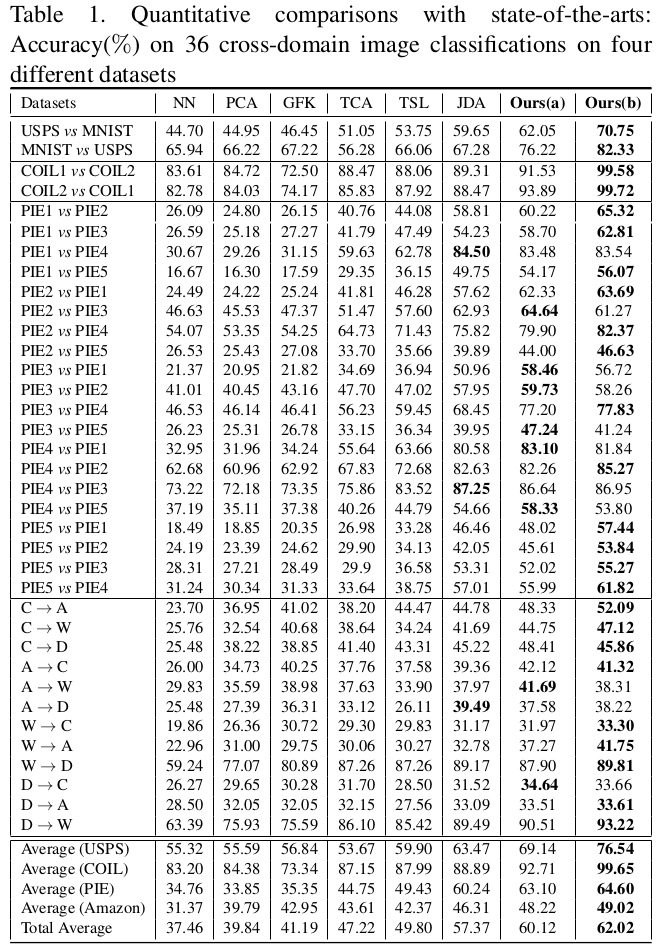
Quantitative comparisons
Quantitative comparisons with state-of-the-arts: Accuracy(%) on 36 cross-domain image classifications on four different datasets
Quantitative comparisons with state-of-the-arts:
Accuracy(%) on 36 cross-domain image classifications on four
different datasets
Parameter sensitivity and convergence analysis
Using COIL2 vs COIL1, and C $\rightarrow$ W datasets, we also empirically check the convergence and the sensitivity of the proposed CDDA with respect to the hyper-parameters. Similar trends can be observed on all the other datasets.
Parameter sensitivity and convergence analysis: (a) accuracy w.r.t $\#$iterations; (b) accuracy w.r.t regularization parameter $\alpha$. As can be seen there, the performance of the proposed CDDA along with JDA becomes stable after about 10 iterations.
Bibliography
Cassius Dio, 50:5; quoted from Cassius Dio: The
Roman History: The Age of Augustus, (trans.) () Scott-Kilvert I.; reprinted in AA100 Assignment
Booklet (),
Milton Keynes, The Open University, p.18.